Support vector machine model for classification

Beijing Institute of Technology | Ming-Jian Li

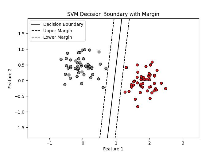
The following Python code is a companion code for the course on Artificial Intelligence and Simulation Science. It functions to establish a support vector machine classification model to classify the given data.

x
1
from sklearn.svm import SVC
2
import numpy as np
3
import matplotlib.pyplot as plt
4

5
# generate data
6
np.random.seed(11)
7

8
mean_1 = [1.8, 0]
9
cov_1 = [[0.1, 0], [0, 0.1]]
10
mean_2 = [0, 0.4]
11
cov_2 = [[0.1, 0], [0, 0.1]]
12

13
X1 = np.random.multivariate_normal(mean_1, cov_1, 50)
14
y1 = np.zeros(50)
15

16
X2 = np.random.multivariate_normal(mean_2, cov_2, 50)
17
y2 = np.ones(50)
18

19
X = np.concatenate((X1, X2), axis=0)
20
y = np.concatenate((y1, y2))
21

22
# support vector classification
23
svc = SVC(kernel='linear')
24
svc.fit(X, y)
25

26
# Plot data
27
plt.scatter(X[:, 0], X[:, 1], c=y, cmap=plt.cm.Set1, edgecolor='k')
28

29
# Plot decision boundary
30
w = svc.coef_[0]
31
b = svc.intercept_[0]
32
x_plot = np.linspace(min(X[:, 0]) - 1, max(X[:, 0]) + 1, 10)
33
y_plot = -w[0] / w[1] * x_plot - b / w[1]
34
plt.plot(x_plot, y_plot, 'k-', label='Decision Boundary')
35

36
# Plot margin
37
margin = 1 / np.linalg.norm(w)
38
b_upper = b + margin
39
b_lower = b - margin
40

41
y_upper = -(w[0] * x_plot + b_upper) / w[1]
42
y_lower = -(w[0] * x_plot + b_lower) / w[1]
43

44
plt.plot(x_plot, y_upper, 'k--', label='Upper Margin')
45
plt.plot(x_plot, y_lower, 'k--', label='Lower Margin')
46

47
# Set the x and y limits for the plot
48
plt.xlim([min(X[:, 0]) - 1, max(X[:, 0]) + 1])
49
plt.ylim([min(X[:, 1]) - 1, max(X[:, 1]) + 1])
50

51
plt.xlabel('Feature 1')
52
plt.ylabel('Feature 2')
53
plt.legend(loc='upper left')
54
plt.title('SVM Decision Boundary with Margin')
55
plt.show()
56

57
X_new = np.array([[2, 0.5], [-1.0, -2.0]])
58
y_pred = svc.predict(X_new)
59

60
print("Predicted Labels:", y_pred)

The result is as follows: