Logistic regression for classification

Beijing Institute of Technology | Ming-Jian Li

The following Python code is a companion code for the course on Artificial Intelligence and Simulation Science. It functions to establish a logistic regression model to classify the given data, with parameters optimized using the gradient descent method.

x
1
import numpy as np
2
import matplotlib.pyplot as plt
3

4
# random seed
5
np.random.seed(42)
6

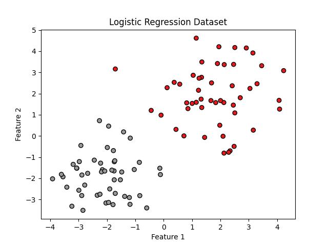
7
# mean value and covariance
8
mean_1 = [2, 2]
9
cov_1 = [[2, 0], [0, 2]]
10
mean_2 = [-2, -2]
11
cov_2 = [[1, 0], [0, 1]]
12

13
# generate samples 
14
X1 = np.random.multivariate_normal(mean_1, cov_1, 50)
15
y1 = np.zeros(50)
16

17
X2 = np.random.multivariate_normal(mean_2, cov_2, 50)
18
y2 = np.ones(50)
19

20
X = np.concatenate((X1, X2), axis=0)
21
y = np.concatenate((y1, y2))
22

23
plt.scatter(X[:, 0], X[:, 1], c=y, cmap=plt.cm.Set1, edgecolor='k')
24
plt.xlabel('Feature 1')
25
plt.ylabel('Feature 2')
26
plt.title('Logistic Regression Dataset')
27
plt.show()
28

29
def sigmoid(z):
30
    y = 1.0/(1.0+np.exp(-z))
31
    return y
32

33
class LogisticRegression:
34
    def __init__(self, learning_rate=0.01, num_iterations=1000):
35
        self.learning_rate = learning_rate
36
        self.num_iterations = num_iterations
37
        self.weights = None
38
        self.bias = None
39

40
    def fit(self, X, y):
41
        num_samples, num_features = X.shape
42

43
        # initialize
44
        self.weights = np.zeros(num_features)
45
        self.bias = 0
46

47
        # gradient descent
48
        for _ in range(self.num_iterations):
49
            linear_model = np.dot(X, self.weights) + self.bias
50
            y_pred = sigmoid(linear_model)
51

52
            dw = (1 / num_samples) * np.dot(X.T, (y_pred - y))
53
            db = (1 / num_samples) * np.sum(y_pred - y)
54

55
            self.weights -= self.learning_rate * dw
56
            self.bias -= self.learning_rate * db
57

58
    def predict_prob(self, X):
59
        linear_model = np.dot(X, self.weights) + self.bias
60
        y_pred = sigmoid(linear_model)
61
        return y_pred
62

63
    def predict(self, X, threshold=0.5):
64
        y_pred_prob = self.predict_prob(X)
65
        y_pred = np.zeros_like(y_pred_prob)
66
        y_pred[y_pred_prob >= threshold] = 1
67
        return y_pred
68

69
logreg = LogisticRegression()
70

71
logreg.fit(X, y)
72

73
X_new = np.array([[2.5, 2.5], [-6.0, -4.0]])
74
y_pred_prob = logreg.predict_prob(X_new)
75
y_pred = logreg.predict(X_new)
76

77
print("Predicted Labels:", y_pred)

The dataset is as follows:

The classification results for the given two points [2.5, 2.5] and [-6.0, -4.0] are:

Predicted Labels: [0. 1.]