Linear regression with gradient descent

Beijing Institute of Technology | Ming-Jian Li

The following Python code is a companion code for the course on Artificial Intelligence and Simulation Science. It functions to fit a curve using linear regression based on a given dataset and make predictions, with parameter optimization using the gradient descent method.

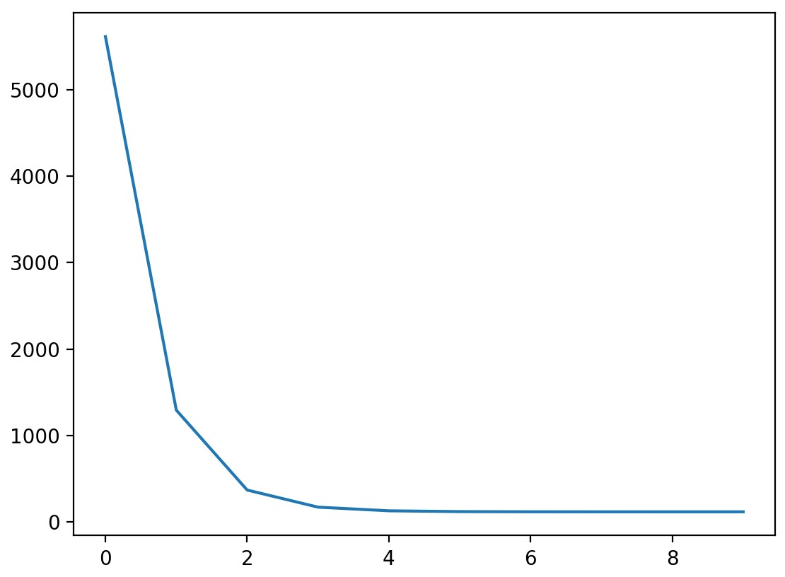
1
import numpy as np
2
import matplotlib.pyplot as plt
3
 
4
# prepare data
5
data = np.array([[32, 31], [53, 68], [61, 62], [47, 71], 
6
                 [59, 87], [55, 78], [52, 79], [39, 59], 
7
                 [48, 75], [52, 71], [45, 55], [54, 82], 
8
                 [44, 62], [58, 75], [56, 81], [48, 60], 
9
                 [44, 82], [60, 97], [45, 48], [38, 56],
10
                 [66, 83], [65, 118], [47, 57], [41, 51], 
11
                 [51, 75], [59, 74], [57, 95], [63, 95], 
12
                 [46, 79], [50, 83]])
13
 
14
x = data[:, 0]
15
y = data[:, 1]
16
 
17
# define loss function
18
def compute_cost(w, b, data):
19
    total_cost = 0
20
    M = len(data)
21
    # calculate loss, and get average
22
    for i in range(M):
23
        x = data[i, 0]
24
        y = data[i, 1]
25
        total_cost += (y - w * x - b) ** 2
26
    return total_cost / M
27
 
28
# define hyperparameters
29
alpha = 0.0001
30
initial_w = 0
31
initial_b = 0
32
num_iter = 10
33
 
34
# gradient descent algorithm 
35
def grad_desc(data, initial_w, initial_b, alpha, num_iter):
36
    w = initial_w
37
    b = initial_b
38
    # define a list to store all loss values
39
    cost_list = []
40
    for i in range(num_iter):
41
        cost_list.append(compute_cost(w, b, data))
42
        w, b = step_grad_desc(w, b, alpha, data)
43
    return [w, b, cost_list]
44
 
45
def step_grad_desc(current_w, current_b, alpha, data):
46
    sum_grad_w = 0
47
    sum_grad_b = 0
48
    M = len(data)
49
    # sum up
50
    for i in range(M):
51
        x = data[i, 0]
52
        y = data[i, 1]
53
        sum_grad_w += (current_w * x + current_b - y) * x
54
        sum_grad_b += current_w * x + current_b - y
55
    # get current gradient
56
    grad_w = 2 / M * sum_grad_w
57
    grad_b = 2 / M * sum_grad_b
58
    # update w and b
59
    updated_w = current_w - alpha * grad_w
60
    updated_b = current_b - alpha * grad_b
61
    return updated_w, updated_b
62
 
63
# use gradient descent method to get best w and b
64
w, b, cost_list = grad_desc( data, initial_w, initial_b, alpha, num_iter )
65
print("w is: ", w)
66
print("b is: ", b)
67
cost = compute_cost(w, b, data)
68
print("cost is: ", cost)
69
plt.plot(cost_list)
70
plt.show()
71
 
72
# draw a fitting curve
73
plt.scatter(x, y)
74
# give prediction for each x
75
pred_y = w * x + b
76
plt.plot(x, pred_y, c='r')
77
plt.show()

The process of the loss value decreasing is as follows: